Custom vector fields provide a great way to add variety and art direction to everything from POP to FLIP to Pyro to Growth Solvers – but setting them up intuitively can sometimes be a challenge, so I was motivated to build out a few tools to make the process easier. This post is to provide some documentation and explanation for the setup.

You can download the HDAs here:
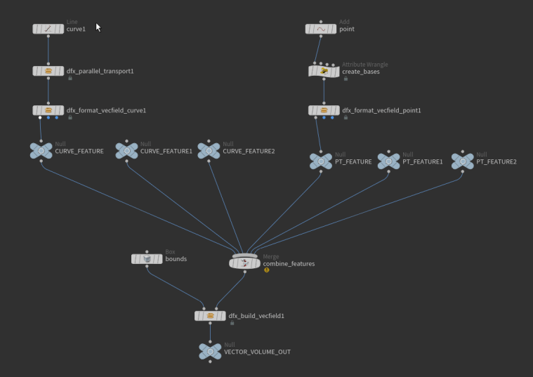
The bundles includes four tools:
The high-level summary:
In effect, these tools allow you to generate ‘features’ in the vector space from points or curves. Features are represented by a set of basis vectors defining their local space, and the effect along each of these bases (e.g., attract vs repel, spin, flow). The overall influence at any given point in space is calculated as a weighted average of these effects (weighted by distance, feature strength, and basis projections).
The basic workflow:
1. Generate and frame your curves and points. A generalized parallel transport HDA is provided to facilitate curve framing, with controls for twisting and resampling.
2. Defined effects for your curves and points (a separate tool is provided for each).
3. Generate your field based on any number of features (or, alternatively, sample the field at specific points).
Documentation:
Parallel Transport
Inputs: a single open or closed curve
Outputs: a framed curve with N, tangent, and bitangent vector attributes.
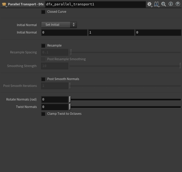
Closed Curve: Toggle on for loops, enabling wrap-around influences for the framing step. Depending on the curve, you may also wish to enable Post Smooth Normals to improve continuity in the neighbourhood of point 0.
Initial Normal: Choose from Set Initial (which takes a user specified starting normal for point 0), or Use First Point (which assumes an existing N attribute on point 0).
Resample & Resample Spacing: Optional resampling of the input curve.
Post Resample Smoothing: Optional smoothing after resampling.
Post Smooth Normals: Applies an attribute blur to N after framing. Useful for some closed curves to better blend in the neighbourhood of point 0.
Rotate Normals: Applies an additional arbitrary rotation of N around the tangent axis. Angles expected in radians.
Twist Normals: Applies an additional twist of N around the tangent axis. Units are number of complete rotations over the length of the curve.
Clamp Twist to Octaves: Enforces integer multiples for Twist Normals. Useful for closed curves.
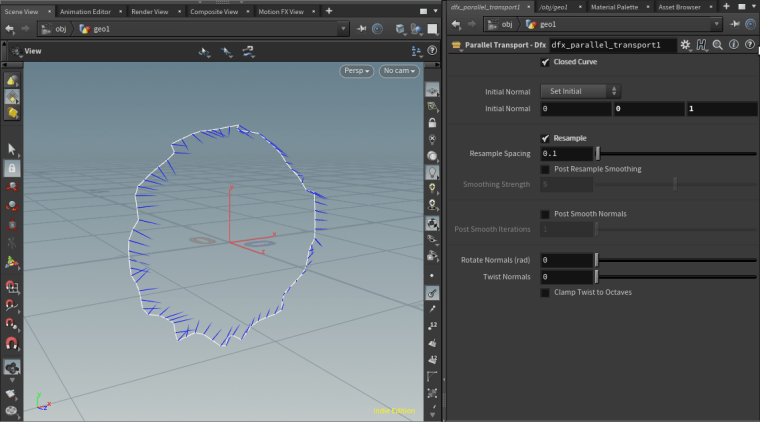
Example workflow:


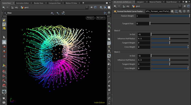
Format Curve Feature
Inputs: A single framed curve, with orthonormal N, tangent, and bitangent vectors.
Outputs: Primary output is a curve feature ready to be passed to Build Vector Field node.
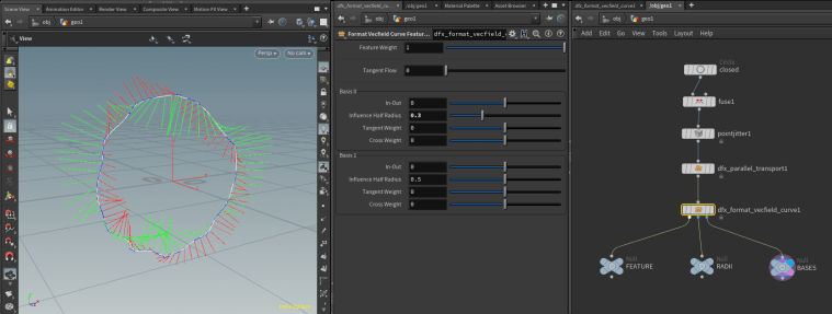
Two visualization outputs also provided:
Output 1 visualizes influence half radius
Output 2 visualized the basis vectors (scaled by influence half radius)
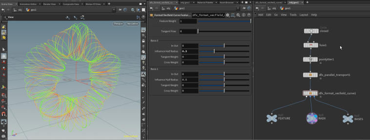
Feature Weight: Overall scaling on the influence of this feature.
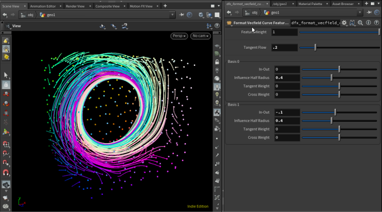
Tangent Flow: How much the vector field should be drawn in the direction of the tangent.
Per-basis settings: (Basis 0 = N, Basis 1 = bitangent)
The behaviour of sampled points reflects a projection-weighted combination of both bases’ effects.
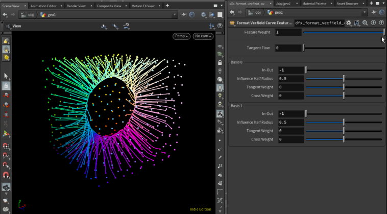
- In-Out: Amount of attraction (negative values) or repulsion (positive values) along this basis.
- Influence Half Radius: Influence weight is scaled by a 1/(1+x^2) kernel, reaching half maximum at this distance along the axis.
- Tangent Weight: Amount of tangent flow from this basis.
- Cross Weight: Rotational influence around the tangent.
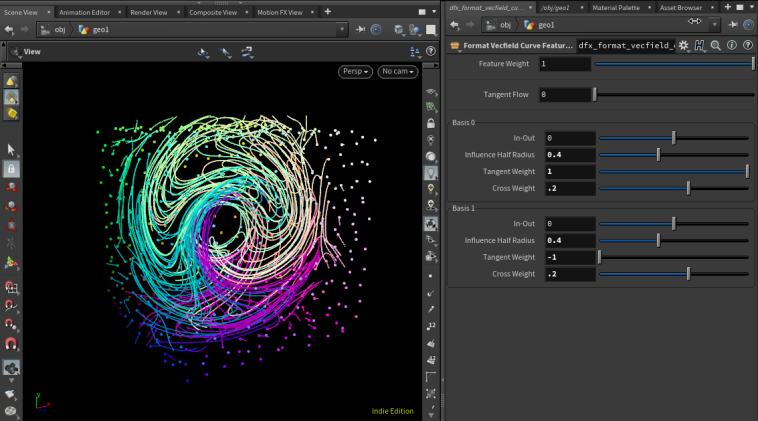
A few example settings for different effects:


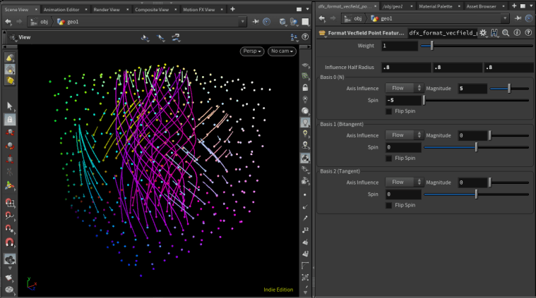
Format Point Feature
Inputs: One or more point, with orthonormal N, tangent, and bitangent vectors. Note: no framing tools are provided for point features, so make sure to provide these vectors!
Outputs: Primary output is a point feature ready to be passed to Build Vector Field node.
Two visualization outputs also provided:
Output 1 visualizes influence half radius
Output 2 visualized the basis vectors (scaled by influence half radius)
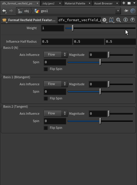
Weight: Overall scaling on the influence of this feature.
Influence Half Radius: Influence weight is scaled by a 1/(1+x^2) kernel, reaching half maximum at this distance along the axis.
Per-basis settings: (Basis 0 = N, Basis 1 = bitangent, Basis 2 = tangent)
- Axis Influence:
- Flow: Movement along direction of the basis
- Attract: Movement toward the point
- Repell: Movement away from the point
- Magnitude: Strength of the effect.
- Spin: Rotation effect around the basis axis.
- Flip Spin: Controls whether the spin effect is influenced by the sign of the projection.
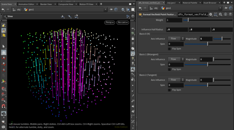
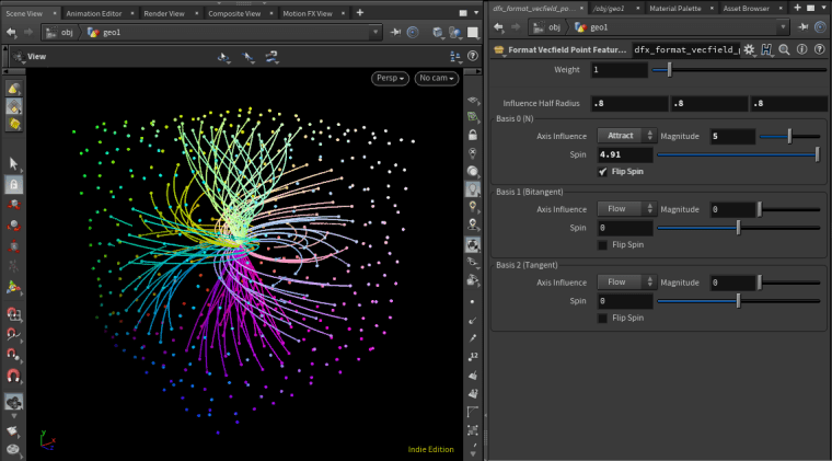
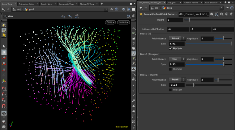
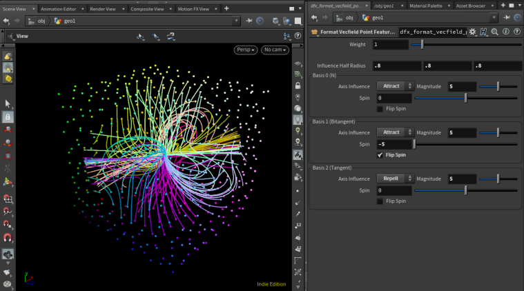
A few example settings for different effects:
Build Vector Field
Input 1 (volume bounds): For ‘Create Volume’ mode, the region in which to generate the vector volume. For ‘Sample Points’ mode, the points at which to generate vectors.
Input 2 (features): All curve and point features whose influence is to be calculated.
Output: For ‘Create Volume’ mode, a vector VDB ‘v’. For ‘Sample Points’ mode, the points to be sampled with vector values ‘v’.
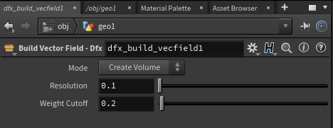
Mode:
Create Volume: Generate a vector VDB.
Sample Points: Calculate vectors only for the input points.
Resolution: Voxel size for VDB. Ignored in ‘Sample Points’ mode.
Weight Cutoff: Minimum influence weight a feature point must have to be included. The default (0.2) corresponds to a distance twice the influence half radius for the feature.
NOTE: The vector field is not scaled! The more features / feature points, the larger these values will be. You will likely want to scale the output before use, but the amount of scaling will vary across settings.
I hope you all find these tools useful! I’m happy to entertain feature requests and will post any updates if and when they become available. Happy vectoring!

Leave a comment