A lot of interesting fluid dynamics come from reactions between different types of fluids. Here I show a straightforward and flexible way to set up FLIP sims to accomplish these kinds of reactions – which can include foaming / dissolving, hardening / thickening, expansion, etc.
Glue constraints in bullet are great – they’re fast and cheap – but by default they only break from impacts. Here’s a relatively straightforward way to break glue with arbitrary forces, including fields. Nothing overly complex, so it should be ok for all levels!
In this tutorial I look at a few ways to use fiber properties in the FEM solver to generate procedural motion. First, I cover a noise-driven approach to generating organic churning motion, and cover a bit about hybrid objects and wrinkly skin in FEM. Next, I show how you can use periodic functions and dynamic target constraints to generate inch-worm style locomotion. Finally, I show how you can set up a tentacle system that flexes towards an arbitrary animated target. Fairly straightforward setups throughout – should be ok for all levels!
New tutorial is now live. In this one, I cover a couple approaches to RBD-like fracturing simulations in FLIP. In the first version, I build the sim entirely in FLIP, using per-particle viscosity to emulate pieces. In the second version, I use a standard bullet RBD sim to drive a secondary FLIP sim. Along the way we cover a few other topics, including a quick look at dual rest uvs for texturing fluids. Enjoy!
Custom vector fields provide a great way to add variety and art direction to everything from POP to FLIP to Pyro to Growth Solvers – but setting them up intuitively can sometimes be a challenge, so I was motivated to build out a few tools to make the process easier. This post is to provide some documentation and explanation for the setup.
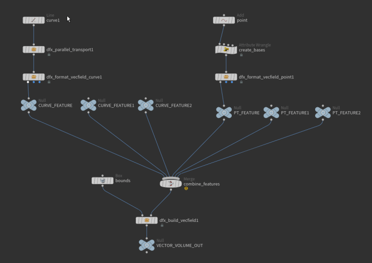
In effect, these tools allow you to generate ‘features’ in the vector space from points or curves. Features are represented by a set of basis vectors defining their local space, and the effect along each of these bases (e.g., attract vs repel, spin, flow). The overall influence at any given point in space is calculated as a weighted average of these effects (weighted by distance, feature strength, and basis projections).
The basic workflow:
1. Generate and frame your curves and points. A generalized parallel transport HDA is provided to facilitate curve framing, with controls for twisting and resampling.
2. Defined effects for your curves and points (a separate tool is provided for each).
3. Generate your field based on any number of features (or, alternatively, sample the field at specific points).
Documentation:
Parallel Transport
Inputs: a single open or closed curve Outputs: a framed curve with N, tangent, and bitangent vector attributes.
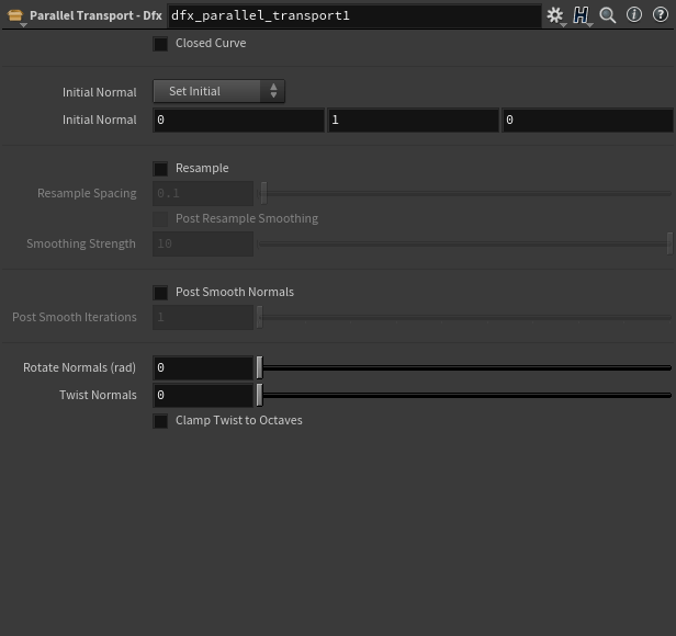
Closed Curve: Toggle on for loops, enabling wrap-around influences for the framing step. Depending on the curve, you may also wish to enable Post Smooth Normals to improve continuity in the neighbourhood of point 0.
Initial Normal: Choose from Set Initial (which takes a user specified starting normal for point 0), or Use First Point (which assumes an existing N attribute on point 0).
Resample & Resample Spacing: Optional resampling of the input curve. Post Resample Smoothing: Optional smoothing after resampling.
Post Smooth Normals: Applies an attribute blur to N after framing. Useful for some closed curves to better blend in the neighbourhood of point 0.
Rotate Normals: Applies an additional arbitrary rotation of N around the tangent axis. Angles expected in radians.
Twist Normals: Applies an additional twist of N around the tangent axis. Units are number of complete rotations over the length of the curve.
Clamp Twist to Octaves: Enforces integer multiples for Twist Normals. Useful for closed curves.
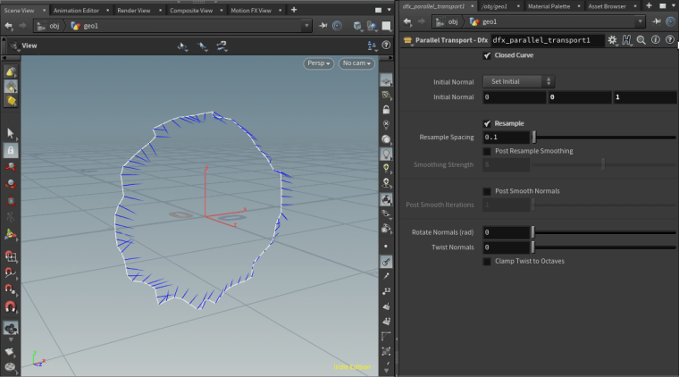
Example workflow:
Defaults with closed curve toggled.Resample.Smooth.Adjust rotation and twist.
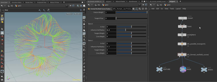
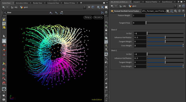
Format Curve Feature
Inputs: A single framed curve, with orthonormal N, tangent, and bitangent vectors.
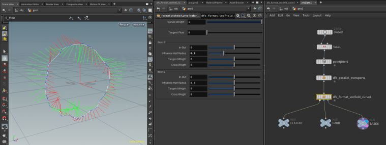
Outputs: Primary output is a curve feature ready to be passed to Build Vector Field node. Two visualization outputs also provided: Output 1 visualizes influence half radius Output 2 visualized the basis vectors (scaled by influence half radius)
Feature Weight: Overall scaling on the influence of this feature.
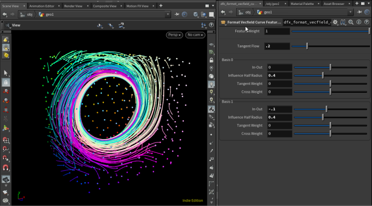
Tangent Flow: How much the vector field should be drawn in the direction of the tangent.
Per-basis settings: (Basis 0 = N, Basis 1 = bitangent) The behaviour of sampled points reflects a projection-weighted combination of both bases’ effects.
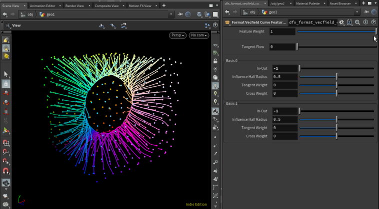
In-Out: Amount of attraction (negative values) or repulsion (positive values) along this basis.
Influence Half Radius: Influence weight is scaled by a 1/(1+x^2) kernel, reaching half maximum at this distance along the axis.
Tangent Weight: Amount of tangent flow from this basis.
Cross Weight: Rotational influence around the tangent.
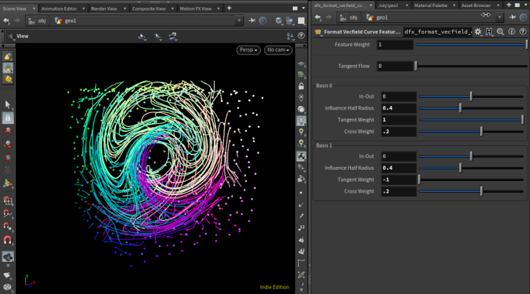
A few example settings for different effects:
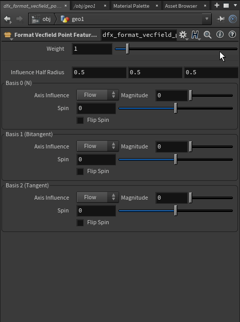
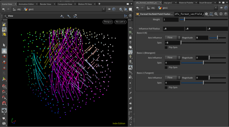
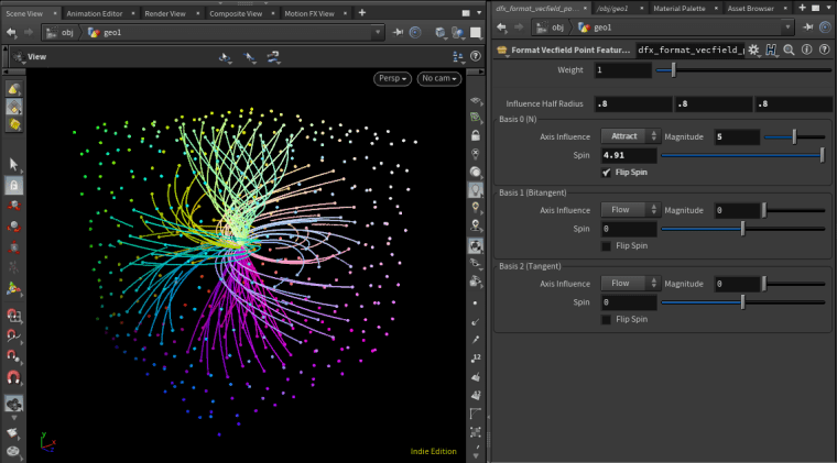
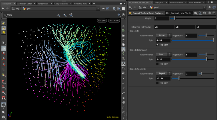
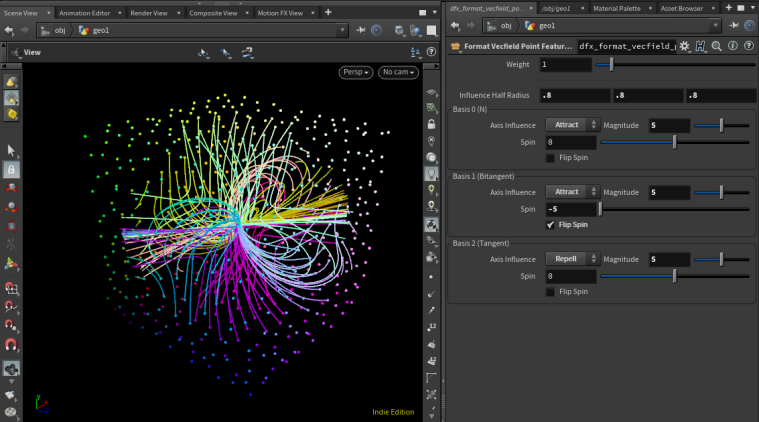
Format Point Feature
Inputs: One or more point, with orthonormal N, tangent, and bitangent vectors. Note: no framing tools are provided for point features, so make sure to provide these vectors!
Outputs: Primary output is a point feature ready to be passed to Build Vector Field node. Two visualization outputs also provided: Output 1 visualizes influence half radius Output 2 visualized the basis vectors (scaled by influence half radius)
Weight: Overall scaling on the influence of this feature.
Influence Half Radius: Influence weight is scaled by a 1/(1+x^2) kernel, reaching half maximum at this distance along the axis.
Flip Spin: Controls whether the spin effect is influenced by the sign of the projection.
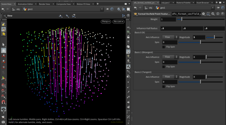
A few example settings for different effects:
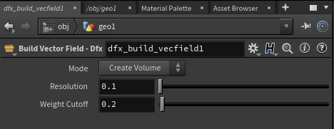
Build Vector Field
Input 1 (volume bounds): For ‘Create Volume’ mode, the region in which to generate the vector volume. For ‘Sample Points’ mode, the points at which to generate vectors.
Input 2 (features): All curve and point features whose influence is to be calculated.
Output: For ‘Create Volume’ mode, a vector VDB ‘v’. For ‘Sample Points’ mode, the points to be sampled with vector values ‘v’.
Mode: Create Volume: Generate a vector VDB. Sample Points: Calculate vectors only for the input points.
Resolution: Voxel size for VDB. Ignored in ‘Sample Points’ mode.
Weight Cutoff: Minimum influence weight a feature point must have to be included. The default (0.2) corresponds to a distance twice the influence half radius for the feature.
NOTE: The vector field is not scaled! The more features / feature points, the larger these values will be. You will likely want to scale the output before use, but the amount of scaling will vary across settings.
I hope you all find these tools useful! I’m happy to entertain feature requests and will post any updates if and when they become available. Happy vectoring!
Just posted another tutorial on how to set up a simulation with Pyro and FLIP solvers interacting. I cover a version where fuel and temperature are sourced from FLIP, while the pyro solver feeds back to consume and advect the FLIP sim, but the general approach can be easily adapted to a variety of different use cases.
Intermediate level. Assumes familiarity with VEX, SOP solvers in DOPs (see here for a refresher!), and some very basic familiarity with FLIP and Pyro in DOPs.
I hope you find it useful and/or interesting, and please comment or drop me a line if you’ve got any questions, ideas for improvements, or any tutorial requests! I’d also love to see anything you make using the setup!
Hip of the workflow (zipped because .hip files aren’t allowed by wordpress):
I’ve had a number of people ask me about this effect, and it’s something people seem to like a lot, so I’ve decided to put together a tutorial and an annotated hip breaking down how it works. The tutorial walks through the ‘standard’ version of the effect, from scratch, then I briefly discuss a few variations – which are also included in the hip!
Beginner/Intermediate level. Assumes basic familiarity with Houdini and VEX, but otherwise nothing wildly complicated!
I hope you find it useful and/or interesting, and please comment or drop me a line if you’ve got any questions, ideas for improvements, or any tutorial requests!
Annotated hip of the workflow (zipped because .hip files aren’t allowed by wordpress):
By popular request, I’ve just put together a tutorial on dynamic fracturing in Houdini. This is a long one (about 2hrs!) and heavy on the VEX and solver logic, but I’ve tried to make sure every step is shown and explained so you can build the whole thing from scratch with enough detail to improvise.
Intermediate/Advanced level. Assumes basic familiarity with Houdini, fracturing workflows, DOPs, and VEX.
As always, I hope you find it useful, and please comment or drop me a line if you’ve got any questions, ideas for improvements, or with any tutorial requests you might have!
I’ve also uploaded an annotated hip of the workflow so you can dig in at your own speed. (Note: zipped because .hip files aren’t allowed by wordpress)
Part 2 of my intro to SOPs in DOPs tutorial is now live! (Part 1 here) In this part, I take a look at fractured geometry, and how to spawn it into live simulations – bringing in geometry and constraints, handling renaming, and avoiding collisions.
Hope you enjoy it – Feel free to comment or drop me a line with any tutorial requests you might have!
Annotated hip of the workflow (zipped because .hip files aren’t allowed by wordpress):
Just uploaded a tutorial covering some of the basics of using the SOPs context inside DOPs. Illustrated with a simple example spawning geometry with dynamic constraints into a bullet sim. I’ll be following up with a part 2 soon!